2024-3S 計算数理演習(東京大学理学部・教養学部) [齊藤宣一] [top] [0] [1] [2] [3] [4] [5] [6] [7] [8] [UTOL]
1. Pythonを用いた数値計算の基礎
まずは単純な計算
Google colaboratoryで,ノートブックを開く.$3+4$ を計算するには,以下のように操作する.
![Out[]](fig/google-colab.png)
ノートブックを開いた直後は,答えが返って来るまでに,やや時間がかかる.2回目以降は,それほど,気にならないはずである.今後,本講義の資料では,上のように入力し,出力が得られることを,次のように書く.In [n]:とOut [n]:が対になっている.
In [1]: 3+4

Out [1]: 7
以下で,いろいろ例示をする.説明はいちいち不要であろう.
In [2]: 3-4

Out [2]: -1
In [3]: 3+(-4)

Out [3]: -1
In [4]: 3*4

Out [4]: 12
In [5]: 3/4

Out [5]: 0.75
In [6]: 12/4

Out [6]: 3.0
In [7]: 12//4

Out [7]: 3
In [8]: 13//4

Out [8]: 3
In [9]: 13%4

Out [9]: 1
In [10]: 3**4

Out [10]: 81
(3^4ではない!)
In [11]: 4**-2

Out [11]: 0.0625
In [12]: 12/4*3

Out [12]: 9.0
In [13]: 12/(4*3)

Out [13]: 1.0
In [14]: (1+2j)*(3+1j)

Out [14]: (1+7j)
すなわち,j は虚数単位 $i$ を表す.3+j とは書かないことに注意せよ.
数値や文字列の出力
これも,例を見ながら色々試して,納得するのが近道である.
In [1]:
x=1.2
print(x)
print(y)

Out [1]:
1.2
---------------
NameError   Traceback (most recent call last)
< ipython-input-27-1faa875c5937 >  in < module >
      1 x=1.2
      2 print(x)
----> 3 print(y)

NameError: name 'y' is not defined
In [2]:
print("x is defined")
print('y is undefined')
print('文字列')

Out [2]:
x is defined
y is undefined
文字列
クォーテーションでもダブルクォーテーションでも同じ(私は,その場の気分で使ってしまうので,ご容赦ください).
In [3]:
s="x is defined"
print(s)
print(type(s))

Out [3]:
x is defined
< class 'str' >
In [4]:
x=10.0
print('x = ',x)
print('x = {}'.format(x))
print(f'x = {x}')

Out [4]:
x = 10.0
x = 10.0
x = 10.0
In [5]:
p=3.141592653589
print(f"{p:.3f}")
print(f"{p:9.3f}")
print(f"p={p:.3f}")
print(f"p={p:9.3f}")

Out [5]:
3.142
    3.142
In [5]:の3行目と5行目では,$p$ の値を表示する際に, 合計9文字のフィールド幅で,小数点以下3桁の数値が右揃えされ,左側がスペースが埋められる. (この場合,小数点も合計の文字数に含まれる.)
In [6]:
x=12.345678
y=41
z='comment'
print(f'real={x:.5f}, integer={y:d}, string={z:s}')
print(f"real={x:.3e}, integer={y:5d}, string={z:s}")
print(f'real={x:.5f}, \n integer={y:d}, string={z:s}')
print(f'real={x:.5f}, \ninteger={y:d}, string={z:s}')

Out [6]:
real=12.34568, integer=41, string=comment
real=1.235e+01, integer=   41, string=comment
real=12.34568,
 integer=41, string=comment
real=12.34568,
integer=41, string=comment
In [7]:
x=12.345678
y=41
z='comment'
print('real={:.5f}, integer={:d}, string={:s}'.format(x, y, z))
print('real={:.3e}, integer={:5d}, string={:s}'.format(x, y, z))

Out [7]:
real=12.34568, integer=41, string=comment
real=1.235e+01, integer=   41, string=comment
In [8]:
x=10.0
y=41
print(f'x = {x}, y = {y}')
print(f'x = {y}, y = {x}')

Out [8]:
x = 10.0, y = 41
x = 41, y = 10.0
変数の型
変数には型というのものがある.
In [1]:
a=1
b=2.0
c=1+2j
print(type(a))
print(type(b))
print(type(c))

Out [1]:
< class 'int' >
< class 'float' >
< class 'complex' >
intは整数型である.Pythonでは「任意」の桁の整数が扱える.floatは,64ビットを用いて表現される,いわゆる倍精度実数型浮動小数点数(binary64)である.これについては,2節で,やや詳しく説明する.しかし,講義を通じて,あまり細かいことは気にしないで,floatは実数型である,くらいに考えれば良い.今後の説明でも,そのように表現する.説明しなくてもわかるであろうが,complexは,2つの実数型の対として表現される複素数型である.(念の為:浮動小数点数=floating point number)
なお,例えば,C言語では,上の意味のfloatをdoubleと書き,floatは単精度実数型浮動小数点数(binary32)を意味している.Pythonでは,言語の仕様としては,単精度はサポートしていないようである.(ただし,数値を単精度で扱うことは可能である.)
上のOut [3]で出力された,str(string)は,文字列である.(数字でないので「型」とは言わない?)
In [2]:
a=1
b=2.0
c=1+2j
x=a+b
y=b+c
print(x)
print(type(x))
print(y)
print(type(y))

Out [2]:
3.0
< class 'float' >
(3+2j)
< class 'complex' >
整数型と実数型の和は実数型になる.実数型と複素数型の和は複素数型になる.差積商にについても同様である.
モジュールの利用
点 $\mathrm{P}(x,y)$ $(x,y>0)$ の偏角を計算を計算するために,次のプログラムを実行する.
In [1]:
x = 10.0
y = 10.0
angle = atan(y/x)
print((angle/pi)*180)

Out [1]:
---------------------------------
NameError                                 Traceback (most recent call last)
<  ipython-input-39-84b2df14c98c > in <  cell line: 3 > ()
      1 x = 10.0
      2 y = 10.0
----> 3 angle = atan(y/x)
      4 print((angle/pi)*180)

NameError: name 'atan' is not defined
Pythonには,あらかじめ様々な関数が定義されている (https://docs.python.org/3/library/functions.html)が, 残念ながら,$\tan^{-1}$ はその中に含まれていない. $\sin,\exp$ なども含まれていない. $\pi$ の値も,そのままでは,利用できない.
特別な関数を利用するためには,モジュール(module)をインポートする必要がある. モジュールとは,Pythonにおいて,特定の機能や目的に応じて関数をまとめる単位のことを言う.
本講義でよく使うのは:
- mathモジュール https://docs.python.org/ja/3/library/math.html
- Numpyモジュール http://www.numpy.org/
- matplotlib.pyplotモジュール https://matplotlib.org/stable/tutorials/introductory/pyplot.html
- Scipyモジュール https://scipy.org/
In [2]:
from math import atan, pi
x = 10.0
y = 10.0
angle = atan(y/x)
print((angle/pi)*180)

Out [2]: 45.0
あるいは,次のように書いても良い.詳しく説明しなくても,利用の仕方は理解できるであろう.
In [3]:
import math
x = 10.0
y = 10.0
angle = math.atan(y/x)
print((angle/math.pi)*180)

Out [3]: 45.0
これは,次のように書くと,より便利である.
In [4]:
from math import *
x = 10.0
y = 10.0
angle = atan(y/x)
print((angle/pi)*180)

Out [4]: 45.0
もちろん指数関数 $\exp$ も利用できる.
In [5]:
from math import exp
x = exp(1)
print(x)

Out [5]: 2.718281828459045
Numpyモジュールにおいても,指数関数expが利用できる.さらに,Numpyでは,リストを引数に与えることができる.
In [6]:
from numpy import exp
x = exp([0, 1, 2])
print(x)

Out [6]: [1.         2.71828183 7.3890561 ]
しかし,mathモジュールでのexpは,引数としてはスカラー値しか受け付けない.
In [7]:
from math import exp
x = exp([0, 1, 2])
print(x)

Out [7]:
-------------
TypeError                                 Traceback (most recent call last)
< ipython-input-45-6808b54d7130 >  in < cell line: 2 > ()
      1 from math import exp
----> 2 x = exp([0, 1, 2])
      3 print(x)

TypeError: must be real number, not list
すなわち,同じ指数関数を計算する,同じ記号の関数expでも,定義されているモジュールが違えば,使い方が異なるのである.
以上を踏まえて,以下の2つを比較せよ.
In [8]:
from numpy import *
from math import *
y=cos(0)
print(y)
x = exp([0, 1, 2])
print(x)

Out [8]:
1.0
---------------------------------------------------------------------------
TypeError                                 Traceback (most recent call last)
< ipython-input-47-fa0ec575be00 > in < cell line: 5 > ()
      3 y=cos(0)
      4 print(y)
----> 5 x = exp([0, 1, 2])
      6 print(x)

TypeError: must be real number, not list
In [9]:
from math import *
from numpy import *
y=cos(0)
print(y)
x = exp([0, 1, 2])
print(x)

Out [9]:
1.0
[1.         2.71828183 7.3890561 ]
前者では,$\cos$ と $\exp$ は,mathモジュールのものが用いられているのに対し, 後者では,numpyモジュールのものが用いられているのである.
これらのことを踏まえて,本講義の例では(すなわち,普通は),モジュールの関数を以下のように利用することにする.
In [10]:
import numpy as np
y=np.cos(0)
print(y)
x = np.exp([0, 1, 2])
print(x)

Out [10]:
1.0
[1.         2.71828183 7.3890561 ]
Google Colaboratoryを使っていると, 意図しないモジュールをロードしたまま, あるいは変数を二重三重に定義して,計算を続けてしまうことがある. このようなことを避けるために,適宜, 次のようにして,モジュールや変数のリセットとすると良い.
In [11]: %reset -f
配列の利用(1次元配列)
1次元配列(ベクトル)の利用の仕方を説明する. それには配列(array)を利用する. 例えば,$\boldsymbol{x}=(1,2,4)$ (横ベクトル)は,次のように定義できる.
In [1]:
x=[1,2,4]
print(x[0])
print(x[1])
print(x[2])

Out [1]:
1
2
4
そうすると,x[0]=1,x[1]=2,x[2]=4となる.すなわち,配列の番号づけは,$0$からはじまる.
しかし,この配列の使い方は薦めない.例えば,
In [2]: 2*x

Out [2]: [1, 2, 4, 1, 2, 4]
というように,あまり嬉しくない計算をされてしまう. 以後,本講義では,numpyの配列(ndarrayクラス)を利用する.
In [3]:
import numpy as np
x=np.array([1,2,4])
print(2*x)
print(type(x))

Out [3]:
[2 4 8]
< class 'numpy.ndarray' >
実際,(いちいち検証しないが)ndarrayクラスの方が,いろいろな数学的操作を,容易かつ高速に実行できる.
次のlinspace関数は,今後とてもよく使う. 閉区間 $[0,5]$ の中に,両端も含めて $6$ の点を等間隔にとり,配列にする場合には,次のようにする.
In [4]:
import numpy as np
x=np.linspace(0,5,6)
print(x)

Out [4]: [0. 1. 2. 3. 4. 5.]
すなわち,z = linspace(a,b,N) とすることで,$\boldsymbol{z}=(z_0,\ldots,z_{N-1})$, $z_k=a+\frac{b-a}{N-1}k$ $(k=0,\ldots,N-1)$を生成する.
In [5]: print(x)
In [6]: len(x)
In [7]: type(x)


Out [5]: [0. 1. 2. 3. 4. 5.]
Out [6]: 6
Out [7]: numpy.ndarray
In [8]: x[6]

Out [8]:
-------------------------------------
IndexError                                Traceback (most recent call last)
< ipython-input-65-04aa5bc9ecce >  in < cell line: 1 > ()
----> 1 x[6]

IndexError: index 6 is out of bounds for axis 0 with size 6
配列のコピーには注意が必要である.例えば,
In [9]:
y=x
print(y)

Out [9]: [0. 1. 2. 3. 4. 5.]
とxをyに「コピー」して,yの第0成分の値を上書きする.
In [10]:
y[0]=-9
print(y)

Out [10]: [-9.  1.  2.  3.  4.  5.]
ここまでは,想像通りであろう.しかし,念の為xの値を確認してみると,
In [11]: print(x)

Out [11]: [-9.  1.  2.  3.  4.  5.]
となり,yを操作しただけなのに,xの値も変わってしまっている.理由を説明すると,それなりに時間がかかるので,ここでは深入りしない.
配列を,文字通りにコピーする際には,copy関数を使うと良い.
In [12]:
print(x)
z=np.copy(x)
print(z)
z[0]=7.8
print(z)
print(x)

Out [12]:
[-9.  1.  2.  3.  4.  5.]
[-9.  1.  2.  3.  4.  5.]
[7.8 1.  2.  3.  4.  5. ]
[-9.  1.  2.  3.  4.  5.]
こんどは,xの値は影響を受けていない.
つぎのような配列の分割もよく使う.
In [13]:
x=np.linspace(11,19,9)
print(x)
y=np.copy(x[1:5])
print(y)
print(x)

Out [13]:
[11. 12. 13. 14. 15. 16. 17. 18. 19.]
[12. 13. 14. 15.]
[11. 12. 13. 14. 15. 16. 17. 18. 19.]
この計算では,配列xを生成したのちに,xの(最初の成分を第0成分と数えて)第1成分から第 $5-1=4$ 成分を,別の配列yにコピーしている.すなわち,x[n:m$+$1]で,配列xの第n成分から第m成分までからなる配列を表す.
なぜ,次のようにしないのか(このようにしても意図するy自体は生成できる),理由は各自で考えよ.
In [14]: y=x[1:5]
グラフの描画
グラフを描画する際には,matplotlib.pyplotモジュール(https://matplotlib.org/stable/tutorials/introductory/pyplot.html)を用いると良い.
例として,$y=x-2x^2$ $(-1\le x \le 1)$のグラフを描いてみよう.そのために linspace関数を用いて, $x_k=-1+\frac{2}{N-1}k$ $(k=0,\ldots,N-1)$を生成して, $y_k=x_k-2x_k^2$を計算し, $(x_k,y_k)$ $(k=0,\ldots,N-1)$を順に線分で結ぶ.
次は,$N=41$に対して,この操作を行うプログラムである.
In [1]:
import numpy as np
import matplotlib.pyplot as plt
x = np.linspace(-1, 1, 41)
y = x - 2.0*x**2
plt.plot(x, y)
plt.show()
![Out[]](fig/exam-fig01.png)
複数のグラフを描画する,線に色をつける,描画方法(実線,破線,マーカーなど)を変える,グリッドを入れる,凡例をつける,軸に説明を入れる,タイトルをつける,などが可能である.詳しくは,「matplotlib color」などで検索せよ.
In [2]:
import numpy as np
import matplotlib.pyplot as plt
x = np.linspace(0, 2*np.pi, 101)
y1 = np.sin(x)
y2 = np.sin(6*x)
plt.plot(x, y1,'r')
plt.plot(x, y2,'b--')
plt.legend(['sin(x)','sin(6x)'])
plt.title('Two functions (sin(x) and sin(6x))')
plt.grid('on')
plt.show()
![Out[]](fig/exam-fig02.png)
In [2]は,次のように書いても全く同じ出力が得られる.
In [3]:
import numpy as np
import matplotlib.pyplot as plt

def func1(t):
    return np.sin(t)

def func2(s):
    m=6.0
    return np.sin(m*s)

x = np.linspace(0, 2*np.pi, 101)
y1 = func1(x)
y2 = func2(x)
plt.plot(x, y1,'r')
plt.plot(x, y2,'b--')
plt.legend(['sin(x)','sin(6x)'])
plt.title('Two functions (sin(x) and sin(6x))')
plt.grid('on')
plt.show()![Out[]](fig/prog-ex1.png)
描画したイメージを自動的に保存する方法を説明する.まず,次を行う.
In [4]:
from google.colab import drive
drive.mount('/content/drive')
すると,(やや間があって)次のようなウインドウが現れるので,次のように進む.
![Out[]](fig/drive1.png)
![Out[]](fig/drive2.jpg)
![Out[]](fig/drive5.jpg)
![Out[]](fig/drive6.jpg)
すると,次のようになる.
In [4]:
from google.colab import drive
drive.mount('/content/drive')
Out [4]:
Mounted at /content/drive
(これは必須ではないが,整理の目的で)Colab Notebooksの下にfigというフォルダを作っておく.
その上で,以下のプログラムを実行すると,Out[2]と同じイメージが,figにsin.pngとして保存される.この他に,例えば,sin.jpgやsin.pdfで保存も可能である.
In [5]:
import numpy as np
import matplotlib.pyplot as plt

x = np.linspace(0, 2*np.pi, 101)
y1 = np.sin(x)
y2 = np.sin(6*x)
plt.plot(x, y1,'r')
plt.plot(x, y2,'b--')
plt.xlabel('x')
plt.ylabel('y')
plt.legend(['sin(x)','sin(6x)'])
plt.title('Two functions (sin(x) and sin(6x))')
plt.grid('on')
plt.savefig("/content/drive/MyDrive/Colab Notebooks/fig/sin.png")
plt.show()
これまでに説明した描画方法は,いわば『pyplotインターフェース』を使用したものである.より,複雑なこと(凝ったこと)をしたい場合には,次のような『オブジェクト指向インターフェース』を利用した方が良い.
In [6]:
import numpy as np
import matplotlib.pyplot as plt

fig, ax = plt.subplots()
x = np.linspace(0, 2*np.pi, 101)
y1 = np.sin(x)
y2 = np.sin(6*x)
ax.plot(x, y1,'r')
ax.plot(x, y2,'b--')
ax.set_xlabel('x')
ax.set_ylabel('y')
ax.legend(['sin(x)','sin(6x)'])
ax.set_title('Two functions (sin(x) and sin(6x))')
ax.grid('on')
plt.savefig("/content/drive/MyDrive/Colab Notebooks/fig/sin.png")
fig.show()
本講義の例では,基本的には『pyplotインターフェース』を用いることにする.必要に応じて,『オブジェクト指向インターフェース』の利用を説明する.
繰り返しと分岐
まずは,for文を説明する.以下の,In [1]からIn [4]までは,全て同じである.
In [1]:
for i in range(10):
    print(i)

Out [1]:
0
1
2
3
4
5
6
7
8
9
In [2]:
for m in range(0,10):
    print(m)
In [3]:
for n in range(0,10,1):
    print(n)
In [4]:
for k in [0,1,2,3,4,5,6,7,8,9]:
    print(k)
for文を用いて, $S_n=\frac{1}{1}+\frac{1}{2}+\frac{1}{3}+\cdots+\frac{1}{n} $ を計算してみよう.以下のIn[5]とIn[6]は,共に,$S_{10}$ を計算している.
In [5]:
n=10
sum=0.0
for i in range(n):
  sum=sum+1.0/(i+1)
print(sum)

Out [5]: 2.9289682539682538
In [6]:
n=10
sum=0.0
for i in range(n):
  sum += 1.0/(i+1)
print(sum)

Out [6]: 2.9289682539682538
すなわち,a+=bは,a+bを新しくaとすること,を意味している.
if文の使い方を,具体例で説明する.
方程式 $f(x)=e^x-2x-1=0$ の(唯一の)正の解 $x=x_*$ を,二分法(bisection method)で計算しよう.初等的な考察により,$1< x_*<2$,かつ,$f(1)<0$,$f(2)>0$ であることがわかる.
まず,$[a_0,b_0]=[1,2]$ とする.そして,$k\ge 0$ に対して,$x_k=\frac{1}{2}(a_k+b_k)$,および, \[ [a_{k+1},b_{k+1}] =\begin{cases} [a_k,x_k] & (f(x_k)f(b_k)\ge 0\mbox{のとき})\\ [x_k,b_k] & (f(x_k)f(b_k)<0\mbox{のとき}) \end{cases} \] と定める.このとき, \[ |x_k-x_*|\le b_{k+1}-a_{k+1}=\left(\frac{1}{2}\right)^{k+1}(b_0-a_0) \] が成り立つ.これより,$|x_k-x_*|\le \varepsilon$ を満たす近似解が欲しい場合には,反復回数が $\displaystyle{k^*= \frac{1}{\log 2}\log\frac{|b-a|}{\varepsilon}}$ 程度必要となることもわかる.
これを実行するのが,次のプログラムである.ただし,1e-7$=10^{-7}$を意味する.
In [7]:
import numpy as np

def func(t):
    return np.exp(t)-2.0*t-1.0

a=1.0
b=2.0
eps=1e-7
kmax=int((1.0/np.log(2.0))*np.log((b-a)/eps))
print('k, x, b-a, f(x)')
for k in range(kmax):
  x=0.5*(b+a)
  if func(x)*func(b)<0.0: a=x
  else: b=x
  print(f'{k:2d}, {x:.8f}, {b-a:.8f}, {func(x):.8f}')

Out [7]:
k, x, b-a, f(x)
 0, 1.50000000,  0.50000000,  0.48168907
 1, 1.25000000,  0.25000000,  -0.00965704
 2, 1.37500000,  0.12500000,  0.20507672
(...略...)
20, 1.25643110,  0.00000048,  -0.00000016
21, 1.25643134,  0.00000024,  0.00000020
22, 1.25643122,  0.00000012,  0.00000002
次のプログラムは,上のプログラムと全く同じことをしているが,多少,python風である.
In [8]:
import numpy as np

def func(t):
    return np.exp(t)-2.0*t-1.0

def bisection(a, b, eps):
  kmax=int((1.0/np.log(2.0))*np.log((b-a)/eps))
  print('k, x, b-a, f(x)')
  for k in range(kmax):
    x=0.5*(b+a)
    if func(x)*func(b)<0.0: a=x
    else: b=x
    print(f'{k:2d}, {x:.8f}, {b-a:.8f}, {func(x):.8f}')
  return 0

def main():
  a=1.0
  b=2.0
  eps=1e-7
  bisection(a,b,eps)

if __name__ == '__main__':
  main()

Out [8]:
k, x, b-a, f(x)
 0, 1.50000000,  0.50000000,  0.48168907
 1, 1.25000000,  0.25000000,  -0.00965704
 2, 1.37500000,  0.12500000,  0.20507672
(...略...)
20, 1.25643110,  0.00000048,  -0.00000016
21, 1.25643134,  0.00000024,  0.00000020
22, 1.25643122,  0.00000012,  0.00000002
やや込み入っているので,論理的な塊のみ以下に示す.
![Out[]](fig/prog-ex2.png)
ただし,if __name__ == '__main__':という行は,この講義の範囲内では,不要である.しかし,今後,作成したプログラムをモジュールとして,あるいは,単独のなんとか.pyとして使用する際に,付けておいた方が良い(というか,付けておく必要がある).なお,今後(次回以降)のサンプルプログラムでは,付けないことにする.
繰り返しには,for文の他に,while文も使える.
In [9]:
import numpy as np

def func(t):
    return np.exp(t)-2.0*t-1.0

def bisection(a, b, eps):
  print('k, x, b-a, f(x)')
  k=0
  while b-a>eps:
    x=0.5*(b+a)
    if func(x)*func(b)<0.0: a=x
    else: b=x
    print(f'{k:2d}, {x:.8f}, {b-a:.8f}, {func(x):.8f}')
    k+=1
  return 0

def main():
  a=1.0
  b=2.0
  eps=1e-7
  bisection(a,b,eps)

if __name__ == '__main__':
  main()

Out [9]:
k, x, b-a, f(x)
 0, 1.50000000,  0.50000000,  0.48168907
 1, 1.25000000,  0.25000000,  -0.00965704
 2, 1.37500000,  0.12500000,  0.20507672
(...略...)
20, 1.25643110,  0.00000048,  -0.00000016
21, 1.25643134,  0.00000024,  0.00000020
22, 1.25643122,  0.00000012,  0.00000002
23, 1.25643116,  0.00000006,  -0.00000007
Out [8]では,k=22まで実行されていたが,Out [9]では,k=23まで実行されている.理由を考えよ.
応用:Fourier級数の収束
関数 \[ f(x)=\pi-|x|\qquad (-\pi\leqq x\leqq \pi) \] のFourier級数展開 \[ f(x)=\frac{\pi}{2}+\frac{4}{\pi} \left( \frac{\cos x}{1^{2}}+\frac{\cos 3x}{3^{2}}+\frac{\cos 5x}{5^{2}}+\cdots\right) \] の収束の様子を図示する関数を作成しよう.そのために,第$n+1$項までの部分和 \[ S_n(x)=\frac{\pi}{2}+\frac{4}{\pi} \sum_{k=0}^{n-1}\frac{\cos((2k+1)x)}{(2k+1)^2} \] を考える.次のプログラムでは,$S_{50}(x)$のグラフを描画している.
In [1]:
import numpy as np
import matplotlib.pyplot as plt

def func(x,n):
  val = 0.0
  for k in range(n):
    theta=(2*k+1)*x
    val += np.cos(theta)/((2*k+1)**2)
  return np.pi/2.0 + (4.0/np.pi)*val

x = np.linspace(-1.5*np.pi, 1.5*np.pi, 100)
y = func(x,50)
plt.figure(figsize=(10, 10))
plt.plot(x, y,'b')
plt.title('convergence of Fourier series')
plt.grid('on')
plt.gca().set_aspect('equal', adjustable='box') # set aspect ratio as 1:1
plt.show()![Out[1]](fig/four1.png)
さらに,$S_{1}(x)$,$S_{10}(x)$,$S_{20}(x)$,$S_{50}(x)$のグラフを並べて描き,収束の様子がよりわかりやすようにしてみよう.
In [2]:
import numpy as np
import matplotlib.pyplot as plt

def func(x,n):
  val = 0.0
  for k in range(n):
    theta=(2*k+1)*x
    val += np.cos(theta)/((2*k+1)**2)
  return np.pi/2.0 + (4.0/np.pi)*val

def drawing(m):
  x = np.linspace(-1.5*np.pi, 1.5*np.pi, m)
  y1 = func(x,1)
  y2 = func(x,10)
  y3 = func(x,20)
  y4 = func(x,50)
  plt.figure(figsize=(10, 10)) # this can be dropped
  plt.plot(x, y1,'b')
  plt.plot(x, y2,'g')
  plt.plot(x, y3,'c')
  plt.plot(x, y4,'m')
  plt.legend(['n=1','n=10','n=20','n=50'])
  plt.title('convergence of Fourier series')
  plt.grid('on')
  plt.gca().set_aspect('equal', adjustable='box') # set aspect ratio as 1:1
  plt.show()
  return 0

def main():
  m=100
  drawing(m)

if __name__ == '__main__':
main()![Out[2]](fig/four2.png)
線形代数学の演算
まずは,ベクトルの内積から.In [1]: import numpy as np a=np.array([1,2,3,4]) b=np.array([5,6,7,8]) c=np.inner(a,b) d=np.dot(a,b) print(a) print(b) print(c) print(d) Out [1]: [1 2 3 4] [5 6 7 8] 70 70
In [2]:
import numpy as np
a=np.array([1+2j,2-1j])
b=np.array([2+1j,1+1j])
c=np.inner(a,b)
d=np.dot(a,b)
e=np.vdot(a,b)
print(a)
print(b)
print(c)
print(d)
print(e)

Out [2]:
[1.+2.j 2.-1.j]
[2.+1.j 1.+1.j]
(3+6j)
(3+6j)
(5+0j)
すなわち,$\boldsymbol{x}=(x_1,\ldots,x_n)$ と $\boldsymbol{y}=(y_1,\ldots,y_n)$ に対して, これらが複素ベクトルであっても,innerとdotでは,$\sum_{i=1}^nx_iy_i$ を計算する.一方で, vdotは,(複素ベクトルに対して,期待通りに)$\sum_{i=1}^nx_i\overline{y_i}$ を計算する.
ベクトルのノルムの値は,次のように計算できる.
In [3]:
import numpy as np
a=np.array([1,0,-3])
x=np.linalg.norm(a,ord=1)
y=np.linalg.norm(a,ord=2)
z=np.linalg.norm(a,ord=np.inf)
w=np.linalg.norm(a,ord=0)
print(x)
print(y)
print(z)
print(w)

Out [3]:
4.0
3.1622776601683795
3.0
2.0
すなわち,$1\le p<\infty$ と $\boldsymbol{x}=(x_1,\ldots,x_n)$ に対して, \[ \|\boldsymbol{x}\|_p=\left(\sum_{i=1}^n |x_i|^p\right)^{1/p} \] の値は,linalg.norm(a,ord=p)で計算できる. \[ \|\boldsymbol{x}\|_\infty=\max_{1\le i\le n}|x_i| \] の値は,linalg.norm(a,ord=np.inf)で計算できる. さらに,linalg.norm(a,ord=0)は,ベクトル $\boldsymbol{x}$ の非零成分の個数を計算する.
次のように使うと便利である.
In [4]:
import numpy as np
from numpy import linalg as la
a=np.array([1,0,-3])
x=la.norm(a,ord=2)
print(x)

Out [4]: 3.1622776601683795
numpyのndarrayクラスでは,2次元の配列,すなわち,行列も利用できる.
In [5]:
import numpy as np
A=np.array([[1,2,3],[5,6,7]])
print(type(A))
print(A)

Out [5]:
< class 'numpy.ndarray' >
[[1 2 3]
 [5 6 7]]
転置とエルミート転置は,次のようにする.
In [6]:
import numpy as np
A=np.array([[1, 2-1j],[3+2j, 4]])
D=A.T
E=A.conj().T
print(D)
print(E)

Out [6]:
[[1.+0.j 3.+2.j]
 [2.-1.j 4.+0.j]]
[[1.-0.j 3.-2.j]
 [2.+1.j 4.-0.j]]
和と差,スカラー倍,行列同士の積は次のように計算する.
In [7]:
import numpy as np
A=np.array([[1,2,3],[4,5,6],[-1,2,1]])
B=np.array([[0,-2,-1],[2,3,4],[2,1,1]])
C=A+B
D=A-B
E=3.0*A
F=A*B
G=np.dot(A,B)
print('A+B=\n',C)
print('A-B=\n',D)
print('3A=\n',E)
print('A*B=\n',F)
print('AB=\n',G)

Out [7]:
A+B=
 [[ 1  0  2]
 [ 6  8 10]
 [ 1  3  2]]
A-B=
 [[ 1  4  4]
 [ 2  2  2]
 [-3  1  0]]
3A=
 [[ 3.  6.  9.]
 [12. 15. 18.]
 [-3.  6.  3.]]
A*B=
 [[ 0 -4 -3]
 [ 8 15 24]
 [-2  2  1]]
AB=
 [[10  7 10]
 [22 13 22]
 [ 6  9 10]]
この例でわかる通り,*では,通常の行列の積でなく,行列の成分ごとの積(アダマール積)を計算する.通常の行列の積を計算する場合には,dotを用いる.
なお,通常の行列の積を計算する場合には,dotの他に,matmulや@ も使える.
In [8]:
import numpy as np
A=np.array([[1,2,3],[4,5,6],[-1,2,1]])
B=np.array([[0,-2,-1],[2,3,4],[2,1,1]])
C=np.dot(A,B)
D=np.matmul(A,B)
E=A@B
print(C)
print(D)
print(E)

Out [8]:
[[10  7 10]
 [22 13 22]
 [ 6  9 10]]
[[10  7 10]
 [22 13 22]
 [ 6  9 10]]
[[10  7 10]
 [22 13 22]
 [ 6  9 10]]
しかし,次のことに注意しなければならない. 行列を扱う際には,ndarrayクラスだけでなく,matrixクラスも利用できる. ところが,matrixクラスでは,通常の行列の積が*で,成分毎の積がmultiplyで計算されてしまう.実際,次のようになる.(matrixクラスとndarrayクラスを*で繋ぐと,通常の行列の積を計算するようである.)ただし,本講義のサンプルプログラムでは,matrixクラスは(多分)使わない.
In [9]:
import numpy as np
A=np.mat('1,2;-5,3')
B=np.mat('3,-1;4,6')
print(type(A))
print(type(B))
print(A*B)
print(np.multiply(A,B))
C=np.array([[1,2],[-5,3]])
D=np.array([[3,-1],[4,6]])
print(type(C))
print(type(D))
print(C*D)
print(type(A*C))
print(A*C)

Out [9]:
< class 'numpy.matrix' >
< class 'numpy.matrix' >
[[11 11]
 [-3 23]]
[[  3  -2]
 [-20  18]]
< class 'numpy.ndarray' >
< class 'numpy.ndarray' >
[[  3  -2]
 [-20  18]]
< class 'numpy.matrix' >
[[ -9   8]
 [-20  -1]]
逆行列と行列式は次のように計算できる.
In [10]:
import numpy as np
A=np.array([[1,2,3],[4,5,6],[-1,2,1]])
B=np.linalg.inv(A)
print(B)
C=np.dot(A,B)
print(C)
a=np.linalg.det(A)
print(a)

Out [10]:
[[-0.58333333  0.33333333 -0.25      ]
 [-0.83333333  0.33333333  0.5       ]
 [ 1.08333333 -0.33333333 -0.25      ]]
[[ 1.00000000e+00 -1.11022302e-16 -5.55111512e-17]
 [ 0.00000000e+00  1.00000000e+00  1.11022302e-16]
 [-4.44089210e-16  1.11022302e-16  1.00000000e+00]]
11.999999999999995
指定したサイズの行列を,各成分を疑似乱数で生成することも可能である. このとき,各成分は $[0,1)$ の中から選ばれる. 一方で,random.randint(p,q,(m,n))では, 各成分が $[p,q]$ の中の整数値をとるような $m\times n$ 行列が生成される.
In [11]:
import numpy as np
A=np.random.rand(3, 4)
B=np.random.randint(10,20,(3,4))
b=np.random.rand(3)
print(A)
print(B)
print(b)

Out [11]:
[[0.90599422 0.44144026 0.95851401 0.35291246]
 [0.89705546 0.47500576 0.7160401  0.17252882]
 [0.75703266 0.94839887 0.26015848 0.06482541]]
[[18 19 18 18]
 [14 17 19 17]
 [16 14 17 18]]
[0.28397206 0.66572637 0.90254491]
零行列と単位行列の生成は重要である.
In [12]:
import numpy as np
A=np.zeros((4,5))
B=np.zeros(4)
C=np.eye(3,5)
D=np.eye(3)
print(A)
print(B)
print(C)
print(D)

Out [12]:
[[0. 0. 0. 0. 0.]
 [0. 0. 0. 0. 0.]
 [0. 0. 0. 0. 0.]
 [0. 0. 0. 0. 0.]]
[0. 0. 0. 0.]
[[1. 0. 0. 0. 0.]
 [0. 1. 0. 0. 0.]
 [0. 0. 1. 0. 0.]]
[[1. 0. 0.]
 [0. 1. 0.]
 [0. 0. 1.]]
何に使うか,ピンと来ないかもしれないが,与えられたベクトルに対して,それを対角行列・subdiagonal(日本語でなんと言う?)な成分とする行列を生成できる.
In [13]:
import numpy as np
M=np.random.rand(4)
A=np.diag(M)
B=np.diag(M, 1)
C=np.diag(M, -1)
print(M)
print(A)
print(B)
print(C)

Out [13]:
[0.30311831 0.94739795 0.07139463 0.09439237]
[[0.30311831 0.         0.         0.        ]
 [0.         0.94739795 0.         0.        ]
 [0.         0.         0.07139463 0.        ]
 [0.         0.         0.         0.09439237]]
[[0.         0.30311831 0.         0.         0.        ]
 [0.         0.         0.94739795 0.         0.        ]
 [0.         0.         0.         0.07139463 0.        ]
 [0.         0.         0.         0.         0.09439237]
 [0.         0.         0.         0.         0.        ]]
[[0.         0.         0.         0.         0.        ]
 [0.30311831 0.         0.         0.         0.        ]
 [0.         0.94739795 0.         0.         0.        ]
 [0.         0.         0.07139463 0.         0.        ]
 [0.         0.         0.         0.09439237 0.        ]]
次は,簡単な応用である(この行列は何?).
In [14]:
import numpy as np
N=5
M=np.ones(N)*2.0
S=np.ones(N-1)*(-1.0)
A = np.diag(M) + np.diag(S, 1) + np.diag(S, -1)
print(A)

Out [14]:
[[ 2. -1.  0.  0.  0.]
 [-1.  2. -1.  0.  0.]
 [ 0. -1.  2. -1.  0.]
 [ 0.  0. -1.  2. -1.]
 [ 0.  0.  0. -1.  2.]]
行列のサイズを取得して,それと同じサイズの行列を作ることができる.
In [15]:
import numpy as np
A=np.random.rand(3, 4)
print('size',A.shape)
print('row',A.shape[0])
print('column',A.shape[1])
B=np.zeros(A.shape)
print(B)
C = np.zeros_like(A)
print(C)

Out [15]:
size (3, 4)
row 3
column 4
[[0. 0. 0. 0.]
 [0. 0. 0. 0.]
 [0. 0. 0. 0.]]
[[0. 0. 0. 0.]
 [0. 0. 0. 0.]
 [0. 0. 0. 0.]]
行列$A$に対して,A[i,:]で$A$の$i$行目のベクトルを,A[:,j]で $A$ の $j$ 列目のベクトルを取得できる.$i$ と $j$ が $0$ から始まることに注意せよ.
In [16]:
import numpy as np
A=np.random.rand(3, 4)
print(A)
print(A[0,:])
print(A[:,2])


Out [16]:
[[0.13570483 0.34920421 0.72672949 0.35033207]
 [0.68598076 0.53217261 0.33295342 0.48206163]
 [0.47258342 0.53856068 0.94639199 0.2131011 ]]
[0.13570483 0.34920421 0.72672949 0.35033207]
[0.72672949 0.33295342 0.94639199]
連立一次方程式を解く際には,次のようにする.説明していなかったが,行列とベクトルの積も@で良い.
In [17]:
import numpy as np
A=np.array([[1,2,-1],[4,5,6],[7,8,-3]])
x=np.ones(3)
b=A@x
print(A)
print(x)
print(b)
xx=np.linalg.solve(A, b)
print(xx)

Out [17]:
[[ 1  2 -1]
 [ 4  5  6]
 [ 7  8 -3]]
[1. 1. 1.]
[ 2. 15. 12.]
[1. 1. 1.]
ただし,大規模な行列を係数行列とする連立一次方程式を解く際には,必ずしも,便利ではないようなので,以後,必要に応じて,他の方法も紹介する.
問題
- 上記の入力と出力をすべて確かめよ.数値を変えて,試してみよ.
- $m\times n$ 実行列と $p\times q$ 実行列の和差積について,いろいろ試してみよ.特に,和差積が定義されていないときに何が起こるのかを,確認せよ.複素行列でも試してみよ.
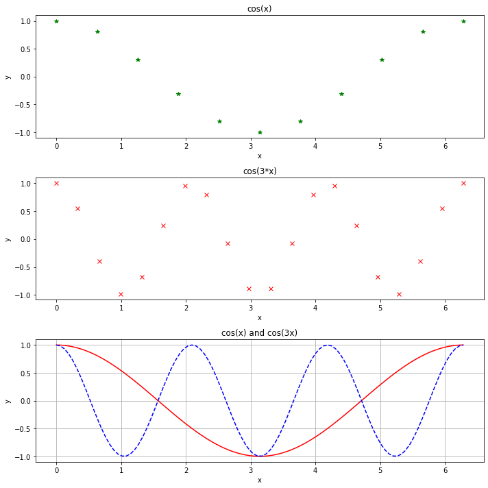
- matplotlib.pyplotモジュールについて,調査せよ.例えば,図1.1のような出力を得ることができるか?(これは,3枚のグラフを縦に並べたものである.subplotなどで調べよ)
課題
課題1.1
関数 \[ f(x)= \begin{cases} 1 & (0 < x < \pi)\\ 0 & (x=-\pi,0)\\ -1 & (-\pi < x < 0) \end{cases} \] のFourier級数展開は, \[ f(x)=\frac{4}{\pi} \sum_{k=0}^\infty \frac{\sin (2k+1)x}{2k+1} \] となる.Fourier級数展開の収束の様子を図示せよ. 具体的には,上の例を参考にして, \[ S_n(x)=\frac{4}{\pi} \sum_{k=0}^{n-1} \frac{\sin (2k+1)x}{2k+1} \] について,例えば,$n=1,10,20,50$などのときのグラフを描画せよ.